
A datasheet says "output ripple < 50 mVpp." The customer puts a brand-new 100 MHz oscilloscope on the output with the long ground lead from the probe kit, captures a screen full of 250 mVpp hash, and emails an angry report: your power supply is 5× out of spec. Nine times out of ten the power supply is fine and the measurement is wrong. The number on the spec sheet was taken under a tightly defined method — a 20 MHz measurement bandwidth, a short ground spring, and a defined load — and the customer reproduced none of it. The difference between "fail" and "pass" here is not a better capacitor; it is PARD measurement discipline.
This guide explains how output ripple and noise (PARD) is actually defined and measured on switching power supplies and adapters: what the 20 MHz bandwidth limit means and why it exists, how to probe the output without manufacturing fake spikes, what the real industry target numbers are, how output filtering produces those numbers, and the pitfalls that turn a compliant supply into a false reject.
What PARD Means: Periodic and Random Disturbance Defined
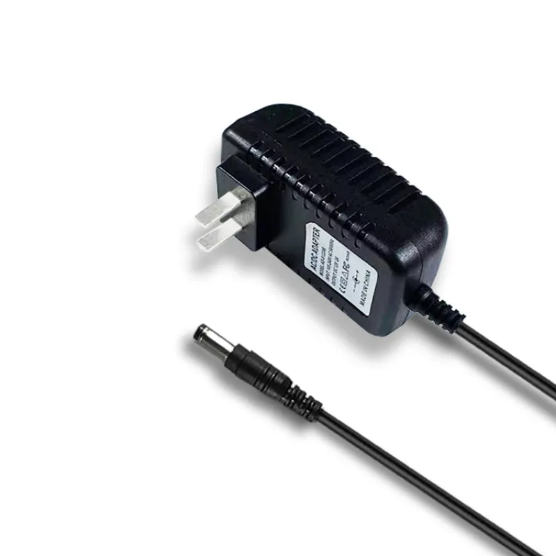
PARD stands for Periodic And Random Disturbance — the umbrella term for everything riding on top of the DC output that isn't DC. It has two distinct halves:
- Periodic — the repeating components. The low-frequency mains ripple at twice the line frequency (100 Hz on a 50 Hz grid, 120 Hz on 60 Hz) that leaks through the bulk capacitor, plus the switching-frequency ripple at the converter's operating point (typically 50–500 kHz) and its harmonics.
- Random — the non-repeating components. High-frequency switching spikes in the MHz range from MOSFET turn-off, output diode reverse recovery, and transformer leakage-inductance ringing, plus disturbances triggered by load transients.
PARD is almost always quoted as a peak-to-peak voltage in millivolts (mVpp), because the spikes — not the RMS average — are what upset a sensitive load. Crucially, PARD is not the same thing as voltage regulation (a DC shift) or transient response (a step event); it is the AC garbage on a steady output at a steady load. Those three are independent specs, compared in detail later in this guide.
Why 20 MHz Is the Industry-Default Measurement Bandwidth
Almost every credible ripple spec is taken with the oscilloscope's 20 MHz bandwidth limit switched on. This is not a trick to hide noise — it is how you measure the real output instead of an antenna.
Above ~20 MHz, what a probe captures is dominated by pickup and self-resonance: the loop formed by the probe tip and its ground return acts as a small antenna, and the probe/scope front end rings. Open the full 100 MHz (or 1 GHz) bandwidth and you measure the measurement system, not the power supply. The 20 MHz limit defines a repeatable window that captures all the energy a real downstream load actually responds to — bulk ripple, switching ripple, and the leading edge of switching spikes — while rejecting the radiated hash that no decoupling network at the load would ever pass.
This 20 MHz convention is written into the major methods: the JEITA RC-9131C standard from the Japan Electronics and Information Technology Industries Association, Intel's ATX 12V / ATX 12VO power supply design guides, and the SSI server-PSU specifications all specify a 20 MHz limit (with a defined termination). Measuring without it is the single most common cause of a false over-spec reading.
Oscilloscope Probe Technique: Ground Spring, Loop Area, and the MLCC Tip
How you connect the probe matters more than the probe's price tag. The rules:
- Kill the ground lead. The 6-inch alligator ground wire from a standard 10× probe kit adds roughly 150–250 nH of inductance that resonates with the scope input and the probe capacitance, manufacturing spikes that aren't on the output. Replace it with a ground spring (the short coil tip accessory) and keep the probe-tip loop area under ~1 inch².
- Use the right probe. A 1× passive probe gives low attenuation and good low-noise reading for ripple amplitude but has limited bandwidth; a 10× passive probe with a ground spring is the everyday choice; a FET / active probe offers very high bandwidth and low loading where the fast spike edge must be seen. Match the probe to what you're characterizing.
- AC-couple the input. A 12 V rail with 50 mVpp of ripple is a tiny AC signal on a large DC pedestal. Leave the scope on DC coupling and the DC level eats the vertical range; switch to AC coupling (or use a blocking cap) so you can zoom the vertical scale onto the ripple.
- Add an MLCC at the tip. Tacking a small MLCC (e.g., 1 µF) right at the measurement point mimics the local decoupling a real load presents and intercepts probe-induced spikes — measure both with and without it to understand what the load will actually see.
For the JEITA/SSI methods, a 50 Ω coaxial termination is often specified to define source impedance; a high-impedance tip is used for amplitude reads. Either way, the ground return is the variable that decides your result.
Measurement Standards Compared
Different industries pin down PARD with different bandwidths, loads, and measurement points. The numbers only mean something alongside their method:
| Standard / guide | Bandwidth limit | Load condition | Measurement point | Termination |
|---|---|---|---|---|
| JEITA RC-9131C | 20 MHz | Rated load (defined %) | Output terminal, defined cable | 50 Ω coax + tip cap |
| Intel ATX 12V Design Guide | 20 MHz | Full / max continuous | Connector / load board | Scope tip with ground spring |
| Intel ATX 12VO (single rail) | 20 MHz | 12 V rail at rated/standby | Mainboard connector | Tip cap + short return |
| EN 50530 (PV inverter) | per method (≤ defined) | MPP operating range | DC input/output port | Defined per test |
The throughline: 20 MHz bandwidth, a defined load, and a short, controlled ground return. Quote a ripple number without those three and it is unverifiable.
Typical PARD Targets by Application
What counts as "good" PARD depends entirely on the load. Tighter is not free — it costs filter volume, post-regulation, or both. Typical industry targets (peak-to-peak, 20 MHz):
| Application | Rail | Typical PARD target | Notes |
|---|---|---|---|
| USB-PD adapter | 5–48 V (PPS/EPR) | ≤ 100 mVpp | USB-PD spec; PPS modes can be tighter |
| Standard ATX 12V | +12 V | ≤ 120 mVpp | Intel ATX 12V guide |
| ATX 3.3 V / 5 V rails | +3.3 V / +5 V | ≤ 50 mVpp | Lower-voltage logic rails |
| Medical (IEC 60601) | varies | ≤ 50 mVpp | Clean rail for sensitive instrumentation |
| Industrial 24 V / 48 V | +24 V / +48 V | ≈ 1% of Vout | ~240 mVpp at 24 V, application-driven |
| High-precision instrument | regulated | < 10 mVpp | Usually needs a post-regulator LDO |
Note the industrial "1% of Vout" rule of thumb produces a larger absolute number at higher voltage, while a precision instrument rail under 10 mVpp almost always needs a linear post-regulator after the switcher.
Output Filter Topology: Low-ESR Electrolytic + MLCC + π/LC
PARD is shaped by the output filter, and the key insight is that no single capacitor covers the whole spectrum:
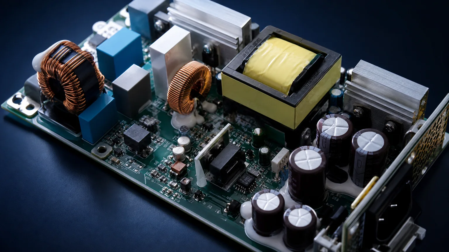
- The low-ESR electrolytic capacitor (105 °C long-life types) handles the bulk and switching-frequency ripple. Its ESR sets the ripple floor — ripple ≈ I_ripple × ESR — which is why "low-ESR" matters more than raw capacitance here. Above roughly 100 kHz, electrolytics lose effectiveness as their impedance becomes inductive.
- MLCC ceramics (e.g., several 22 µF X7R in parallel) take over above 100 kHz and snub the high-frequency hash the electrolytic can no longer touch. This is the "finishing" stage that kills the spike content.
- A π-section (C–L–C) or second-order LC filter adds a further roll-off for demanding rails, and a post-regulator LDO is the last resort when single-digit-mVpp output is required.
The division of labor mirrors input EMI filtering, where bulk and ceramic parts also split duties by frequency — see our LLC resonant vs hard-switched topology selection guide for how the converter topology itself sets how much ripple the filter must clean up, and our X/Y safety capacitor EMI filter guide for the input-side dual of this output-side filtering.
How Load Conditions Change PARD
PARD is not one number — it moves with the operating point, which is why the standards fix the load:
- Light load (10%) can show higher ripple, not lower. Many converters drop into discontinuous conduction mode (DCM) or pulse-skipping/burst mode at light load, producing larger, irregular ripple bursts than at nominal load.
- Nominal load (50%) is the cleanest, best-behaved operating point.
- Full load (100%) typically shows the highest continuous switching ripple because the ripple current is largest.
- A dynamic step (50→100%) with a defined dI/dt tests transient response, a different spec — the momentary dip and recovery, not the steady-state PARD.
Input voltage matters too: at 90 VAC the bulk capacitor sees deeper discharge between mains peaks than at 264 VAC, so the 100/120 Hz twice-line ripple component is larger at low line. Measuring only at 50% nominal load and high line flatters the result and hides the DCM and low-line cases.
Where the Noise Comes From: Switching Spikes and Reverse Recovery
The high-frequency, random part of PARD has identifiable sources, and knowing them is half the cure:
- MOSFET turn-off spike — the switch node Vds rings as the device turns off into circuit parasitics; this couples through the transformer to the output as a fast spike.
- Output diode reverse recovery (trr) — as the rectifier commutates, its stored charge produces a sharp current snap and a corresponding voltage spike (often tamed with a snubber or a Schottky/SiC rectifier).
- Transformer leakage-inductance ringing — leakage energy rings at tens of MHz, the classic source of high-frequency hash on the output.
These are exactly the MHz-range events the 20 MHz bandwidth limit partially attenuates — which is why the leading edge still shows but the radiated overshoot does not. They are real, but the load only responds to the energy below ~20 MHz.
Common-Mode vs Differential-Mode Output Noise
A subtle source of false ripple readings is mixing up two different noise modes on the output:
- Differential-mode noise is the voltage difference between the two output terminals (V+ to V−) — this is the ripple the load actually sees and what the spec means by PARD.
- Common-mode noise is the voltage that both output terminals share with respect to earth/chassis, driven by the primary-to-secondary coupling capacitance of the transformer. If your probe ground references chassis while the output floats, common-mode noise gets added into your reading and inflates the apparent ripple.
Common-mode output noise is usually clamped with a small output Y-capacitor (e.g., 1 nF) returning CM current, while differential ripple is the job of the bulk + MLCC filter. Separate the two before judging a number: measure differentially across the load, not output-to-chassis.
PARD vs Line/Load Regulation vs Transient Response
These four specs are routinely confused, yet they measure completely different behaviors. PARD is AC noise at a fixed steady state; the others describe DC accuracy and dynamic recovery:
| Spec | What it measures | Stimulus | Typical unit |
|---|---|---|---|
| PARD (ripple & noise) | AC content on the DC output at steady state | None (steady load/line) | mVpp |
| Line regulation | DC output shift vs input voltage change | Vin sweep (e.g., 90→264 VAC) | % or mV |
| Load regulation | DC output shift vs load change | Static load change (e.g., 10→100%) | % or mV |
| Transient response | Momentary dip + recovery time to a load step | Dynamic step with defined dI/dt | mV dip / µs |
A supply can have excellent regulation and still have poor PARD, or vice versa. When a spec sheet quotes a single "ripple" line, confirm it is steady-state PARD at a defined load and bandwidth — and check the other three separately.
Five Common PARD Measurement Pitfalls
- Measuring at full 100 MHz bandwidth. The most frequent false reject — the open bandwidth captures probe self-resonance and radiated antenna pickup as "ripple." Switch on the 20 MHz limit before drawing any conclusion.
- Using the long 6-inch ground clip. That alligator lead adds ~200 nH that resonates with the scope's input and the probe capacitance, producing fake spikes that aren't on the output. Use a ground spring and keep the loop under 1 inch².
- Leaving the scope on DC coupling. A 12 V rail's DC level fills the vertical range, so the 50 mVpp ripple can't be resolved. AC-couple (or block the DC) and zoom in.
- No MLCC bypass at the probe tip. Without a small tip capacitor mimicking real load decoupling, you read probe-induced spikes the actual load would never see — and may over-spec the supply.
- Ignoring mode separation and load range. Measuring output-to-chassis folds common-mode noise into the reading, and testing only at 50% misses the light-load DCM case where ripple can be worst. Also re-test after aging: an electrolytic's ESR rises over life, raising ripple — a unit that passed new can drift out of spec, which ties directly to capacitor wear-out modeling in our power supply MTBF reliability calculation guide.
Sanyi Power Supply Ecosystem — PARD Designed to the Right Standard
Sanyi designs its USB-PD, desktop, industrial and medical power lines to application-correct PARD targets verified under the proper 20 MHz method, not to a flattering full-bandwidth number. Each output stage pairs a low-ESR 105 °C electrolytic for bulk and switching ripple with parallel MLCC ceramics for the high-frequency hash, stepping up to π/LC sections or a post-regulator where a rail demands single-digit mVpp. The HP high-power adapter series (up to 240W) carries the output filtering to hold ripple targets at full load, and the APN desktop adapter series applies the same discipline across mid-power desktop and IT loads. For dense multi-port charging, the SY-C260W multi-mode charger and the higher-output SY-C500W high-power charger balance fast GaN switching against the output ripple budget.
Because output noise quality is a system trade-off — topology, filter, layout and load all at once — our supplies are characterized to the standard your application actually cites. Contact our power engineering team with your rail voltages, PARD target, load profile and destination standard, and we will recommend a platform with the matching output-filter scheme.
FAQ
Why measure at 20 MHz instead of the full 100 MHz? Because above ~20 MHz the oscilloscope captures probe self-resonance and radiated antenna pickup rather than the supply's real output. The 20 MHz bandwidth limit defines a repeatable window that includes everything a downstream load actually responds to — bulk ripple, switching ripple and the leading edge of spikes — while rejecting hash that no load would ever pass. It is the bandwidth used by JEITA RC-9131C, Intel ATX 12V and SSI specs, so a number taken any other way isn't comparable.
Does a long ground clip really change the reading that much? Yes — dramatically. A 6-inch alligator ground lead adds roughly 150–250 nH of inductance that resonates with the probe and scope input capacitance, manufacturing spikes that are not present on the output. Swapping to a ground spring and keeping the tip loop under ~1 inch² can turn an apparent 250 mVpp "failure" back into the real ~40 mVpp output. The ground return, not the probe price, usually decides the result.
Why is ripple higher at light load than at full load? Many switching converters drop into discontinuous conduction mode (DCM) or pulse-skipping/burst mode at light load, delivering energy in irregular bursts that produce larger, less periodic ripple than smooth continuous conduction at nominal load. That's why standards fix the load condition and why you should test the 10% case, not just 50% — the light-load number is frequently the worst one.
What does the MLCC at the probe tip actually catch? A small ceramic capacitor (e.g., 1 µF) tacked right at the measurement point does two things: it mimics the local high-frequency decoupling a real load presents, and it shunts probe-induced and high-frequency spikes that wouldn't reach the actual load. Measuring with and without it shows the difference between what the load sees and what the probe alone picks up — helping you avoid over-speccing the supply on artifacts.
How is PARD related to EMC conducted emissions? They overlap in frequency but measure opposite things. PARD is the output-port noise quality — the AC content on your own DC rail that your load must tolerate. EMC conducted emissions are noise the supply pushes back onto the AC mains, disturbing other equipment, governed by limits like CISPR 32 / FCC Part 15. The same switching events drive both, but a clean output (good PARD) does not guarantee low mains emissions, and vice versa — they are separate tests with separate fixes.
.webp)