
At 02:14 on a Tuesday, a single power supply inside a colocation rack failed open. The rack carried a customer's entire transaction-processing cluster on one PSU, because the original build had treated power as an afterthought. The cluster went dark for just over four hours while a technician was dispatched, located a spare, and recabled the chassis. The post-incident review put the direct loss north of a million dollars — and the root cause was not a bad supply. The supply's datasheet quoted a 200,000-hour MTBF, perfectly respectable. The fault was architectural: a single point of failure feeding a system that was never allowed to stop. Six months after the rack was rebuilt with N+1 redundancy and hot-swap modules, the operator logged zero power-related downtime.
That story captures the central truth of mission-critical power: you do not buy your way to 99.999% availability with a higher-MTBF single supply. You buy it with redundancy. This guide is a procurement-side walk through N+1, 1+1 and 2N architectures, the hardware that makes hot swap and parallel operation safe, ORing diodes versus ORing MOSFETs, AC and DC redundancy modules, and the design pitfalls that quietly reintroduce the single point of failure you thought you had eliminated.
Why Five-Nines Availability Demands Redundancy, Not a Higher-MTBF Single PSU
A single power supply, no matter how good, has a finite failure rate. MTBF tells you the statistical mean time between failures for one unit, but it says nothing about what happens to the load when that one unit fails: the load goes down, full stop. Doubling the MTBF of a single supply halves the failure frequency but never eliminates the consequence. Redundancy attacks the consequence directly — when one supply fails, another is already carrying or instantly assumes the load, and the system never notices.
This is why a careful reliability program runs two analyses in parallel. The first quantifies how long a single supply is expected to last; we cover that math in our companion power supply MTBF reliability calculation guide. The second — this article — asks how to build an architecture whose availability far exceeds any single component's MTBF. The two are complementary: MTBF sizes the modules, redundancy sizes the system.
The Three Foundations of Redundancy: N+1, 1+1 and 2N
Three architectures cover the overwhelming majority of redundant power designs. N+1 uses N supplies to carry the load plus one extra running in parallel, so any single failure leaves N units still rated for the full load. 1+1 is the simplest special case: one working supply plus one full backup. 2N duplicates the entire power path — two independent strings, each capable of carrying 100% of the load, typically fed from separate utility/UPS feeds (the data-center "A+B feed").
| Architecture | Fault tolerance | Per-PSU load (full system load) | Typical application | Relative cost |
|---|---|---|---|---|
| N+1 | Any 1 module | N/(N+1) ≈ 75–85% | Telecom plant, edge cabinets, industrial racks | Low–medium |
| 1+1 | The 1 working module | ~50% (backup shares or idles) | Single-chassis critical loads | Medium |
| 2N | A full power string | ~50% per string | Tier III/IV data centers, hospitals | High (≈2×) |
N+1 is the workhorse because its overhead shrinks as the system grows: a 7+1 array spends only one-eighth of its capacity on redundancy, while a 1+1 pair spends half.
N+1 Redundancy in Detail
In an N+1 array, all N+1 supplies run simultaneously and share the load. The practical consequence buyers often miss is that every supply runs lighter than its rating. A 3+1 array sized for a load that three units could just carry actually spreads that load across four units, so each runs at roughly 3/4 = 75% during normal operation; a 5+1 array runs each unit near 5/6 ≈ 83%. Lighter loading lowers internal temperatures and, helpfully, extends each unit's own MTBF — redundancy and longevity reinforce each other.
Typical configurations are 3+1, 5+1 and 7+1. The right N is an economic balance: a larger N dilutes the cost of the "+1" but raises the consequence of a second simultaneous failure before the first unit is replaced. This is exactly why hot swap matters — the faster a failed unit is replaced, the shorter the window in which the array is running without margin.
1+1 and 2N Redundancy Compared
1+1 redundancy is electrically a 2N system collapsed into one chassis: two supplies, either of which can carry the full load. It is the cleanest answer for a single critical device — a controller, a core switch, a medical instrument. The limitation is that everything downstream of the shared output bus and the shared chassis is still common.
True 2N removes that commonality by duplicating the entire path: two PSUs, two distribution buses, two upstream feeds, ideally two physical routes. A failure anywhere in string A — including its utility feed, its UPS and its breaker — leaves string B untouched. Tier III and Tier IV data centers effectively mandate this; for the system-level comparison of where 2N PSU strings sit relative to facility UPS topology, see our data center UPS vs industrial UPS selection guide. The trade-off is blunt: 2N roughly doubles capital cost and footprint. You pay for it where downtime is genuinely intolerable, and you choose N+1 where it is merely expensive.
Hot Swap Hardware Requirements
Redundancy is only useful if a failed module can be replaced without taking the system down — that is the entire point of hot swap. Doing it safely requires hardware features that rarely appear on a basic datasheet:
- Make-before-break signal sequencing. Connector pins are staggered so that ground mates first, then bulk power, then signal/enable last. On extraction the order reverses. This prevents the inserted module from yanking the live bus voltage down or back-feeding a half-connected pin.
- Inrush limiting on insertion. A module inserted into a live bus must charge its input capacitance without collapsing the rail. An onboard NTC thermistor or, better, a MOSFET soft-start ramps the inrush instead of presenting a momentary short. Our companion inrush current limiting guide covers the cold-insertion case in depth.
- Power-good signal. A logic output tells the system the freshly inserted module has reached regulation before the controller counts it toward redundancy.
- Gold-plated, sequenced contacts. Hot-plug contacts oxidize and arc; gold plating and a defined mating sequence keep contact resistance stable across thousands of insertions.
Skip any of these and "hot swap" becomes "hot crash."
Two Current-Sharing Methods for Parallel Operation
When supplies run in parallel they must share the load; otherwise the one with the slightly highest output voltage hogs current, overheats and fails first — defeating the redundancy. Two schemes dominate.
Droop (passive) sharing deliberately lets each supply's output voltage sag slightly as its current rises. A unit carrying more current droops more, so the others naturally pick up slack. It is open-loop, needs no interconnect wire, and is cheap — but its accuracy is modest and degrades badly at light load. Active load-share bus sharing connects all units with a single share-bus wire; each unit references the bus to trim its own current toward the average, closing the loop for tight balance.
| Property | Droop (passive) | Active load-share bus |
|---|---|---|
| Sharing accuracy | ±5–10% | ±2–3% |
| Interconnect | None | One share-bus wire |
| Complexity / cost | Low | Medium |
| Light-load behavior | Poor (imbalanced) | Good |
| Typical control IC | Internal voltage-droop | Load-share controllers (e.g. UC3902-class, LM5067-class) |
| Typical application | Low-cost N+1, non-critical | Tight-tolerance N+1, telecom plant |
Control ICs such as the UC3902 and LM5067 families are cited here only as widely documented industry references; Sanyi does not represent or resell those vendors.
ORing Diode vs ORing MOSFET
Paralleled supplies need fault isolation so a shorted unit cannot drag the shared bus down through its own failed output. Historically this was a Schottky ORing diode in each output: it conducts forward current to the bus and blocks reverse current from a failed neighbor. The penalty is its forward drop — roughly 0.5V — which at 10A burns about 5W of continuous heat per leg, demanding heatsinking and stealing efficiency.
The modern answer is an ORing MOSFET managed by a controller (LTC4357-class, LM5050-class) that senses the drain-source voltage and switches a low-Rds(on) MOSFET on for forward conduction, off in microseconds on reverse current. With a few milliohms of Rds(on), the same 10A dissipates milliwatts instead of watts.
| Property | Schottky ORing diode | ORing MOSFET (controller-driven) |
|---|---|---|
| Forward drop / on-resistance | Vf ≈ 0.5 V | Rds(on) ≈ a few mΩ |
| Loss at 10 A | ~5 W (continuous) | ~mW range |
| Thermal design | Heatsink required | Minimal |
| Reverse-blocking speed | Inherent | µs-level controlled turn-off |
| Relative cost | Low | Medium |
| Typical IC | — (passive) | LTC4357-class, LM5050-class |
For any array above a few amps per leg, the MOSFET approach pays back its cost in efficiency and eliminated heat almost immediately. (Controller part numbers are industry references only.)
AC Redundancy Module (ARM) and DC 48V Plant (DRM)
Two module types productize redundancy at the system edges. An AC Redundancy Module (ARM) merges two independent AC feeds at a single supply's input, automatically selecting the live source so the PSU rides through the loss of either utility/UPS feed. A DC Redundancy Module (DRM) combines multiple PSU outputs onto a common DC bus with built-in ORing, the standard building block of a telecom −48V DC power plant where many rectifiers feed one battery-backed bus. If your architecture is a 48V DC plant, the DRM/ORing layer is where module-level redundancy actually lives — the rectifiers come and go, the bus stays up.
Cold Standby vs Hot Standby
The "+1" in N+1 can wait two ways. In cold standby the backup is powered down until a failure is detected, then started — switchover takes milliseconds to seconds and the load must ride through on hold-up capacitance during that gap. In hot standby the backup is always energized and sharing a light load, so takeover is effectively instantaneous (microseconds). Hot standby is the safer choice for true zero-interruption loads, but it only makes economic sense if the backup is efficient at light load. This is precisely where 80 PLUS Titanium matters: Titanium specifies efficiency even at 10% load, so a hot-standby unit idling at light load is not bleeding away the energy savings you bought it for. A supply efficient only near full load makes a poor hot-standby member.
Relating Redundancy to Availability
Availability is usually expressed in "nines," and the jump from one nine to the next is steep. The table below converts each level to allowable annual downtime:
| Availability | "Nines" | Approx. downtime per year |
|---|---|---|
| 99% | Two nines | ~3.65 days |
| 99.9% | Three nines | ~8.77 hours |
| 99.99% | Four nines | ~52.6 minutes |
| 99.999% | Five nines | ~5.26 minutes |
| 99.9999% | Six nines | ~31.5 seconds |
A single supply with a 200,000-hour MTBF cannot reach five nines on its own — its repair time alone blows the budget. But put units in N+1 with fast hot-swap replacement and the system MTBF climbs into the tens of millions of hours, because both units must fail inside the short repair window for the load to drop. Architecturally, redundancy buys availability that no realistic single-unit MTBF improvement can match.
Five Common Redundancy Design Pitfalls
Even good hardware fails when the system around it is wrong. The recurring traps:
- Droop sharing at light load. Passive droop balances acceptably near full load but diverges badly when lightly loaded — one unit can carry most of the current while the others coast, undoing the thermal benefit. Use active sharing where light-load operation is normal.
- Un-cooled ORing diodes. A 0.5V diode at high current is a real heater. Designers who copy a diode ORing scheme without budgeting heatsinking get thermal failures in the protection element.
- Missing hot-swap signal sequencing. Inserting a module without make-before-break ordering momentarily pulls the live backplane down, glitching every other load on the bus.
- Shared-ground EMI loops. Tying redundant supplies through a large common-ground loop injects noise; the redundancy is intact but the system fails EMC.
- Identical-batch common-mode failure. N+1 units from the same lot can share the same latent defect and fail together — defeating statistical independence.
- Hidden upstream SPOF. Redundant PSUs plugged into one outlet, one breaker, or one PDU share a single point of failure no amount of module redundancy can cover. True 2N requires independent feeds all the way up.
Sanyi Power Solutions for Redundant and Parallel Operation
Across Sanyi's adapter and charger lines, models are specified to support clean parallel operation and N+1 redundancy where the application demands continuous uptime. For high-power single-output needs that pair well in 1+1 or N+1 arrays, the HP series high-power adapter delivers a dense 240W building block. For distributed desktop and edge equipment, the APN desktop adapter series offers compact units suited to redundant edge cabinets. Where higher current and multi-stage charging are required, the SY-C260W multi-stage charger and the SY-C500W high-power charger provide the headroom to run lightly loaded in hot-standby roles. Our engineering team can advise on share-bus wiring, ORing selection and breaker coordination for your specific N+1 or 2N topology.
FAQ
Q1: What is the difference between N+1 and 1+1 redundancy?
1+1 is the special case of N+1 where N equals one: a single working supply plus a single full backup, each typically rated for 100% of the load, so one runs at about half capacity. General N+1 spreads the load across N working units plus one spare, so each unit runs at N/(N+1) of its rating (about 75% in a 3+1, 83% in a 5+1) and the redundancy overhead shrinks as the array grows. Choose 1+1 for a single critical device; choose a larger N+1 when many units share a bus and you want the cost of the extra unit amortized across the array.
Q2: Why have ORing diodes been replaced by ORing MOSFETs?
A Schottky ORing diode drops roughly 0.5V forward, so at 10A it dissipates about 5W of continuous heat per leg, hurting efficiency and demanding heatsinking. An ORing MOSFET driven by a dedicated controller presents only a few milliohms of on-resistance, cutting that loss to the milliwatt range while still blocking reverse current in microseconds when a neighbor fails. For any meaningful current the MOSFET approach wins on efficiency, thermals and reliability, which is why modern redundant designs default to it.
Q3: Is droop current sharing accurate enough for a redundant system?
It depends on the load profile. Droop sharing holds roughly ±5–10% balance and is perfectly adequate for cost-sensitive N+1 arrays that normally run near full load. But droop diverges badly at light load, so if your system spends significant time lightly loaded — common in hot-standby and edge applications — the imbalance can overstress one unit. There, active load-share bus sharing (±2–3%) is worth its modest extra cost.
Q4: Can hot swapping damage the power supply or the system?
Not if the hardware is designed for it. Safe hot swap requires make-before-break connector sequencing (ground first, signal last), inrush limiting so the inserted module charges its input capacitance without collapsing the live bus, a power-good signal so the controller only counts a module once it is in regulation, and gold-plated sequenced contacts. A supply lacking these features should not be hot-inserted — doing so can glitch the backplane and disturb other loads.
Q5: Do redundant power supplies have to be the same model?
For parallel current sharing, yes — practically they should be the same model and firmware so their output voltages, droop characteristics and share-bus behavior match; mixing models invites severe current imbalance. The one nuance worth managing is common-mode failure: units from a single production lot can share a latent defect, so for the highest-availability systems some operators deliberately source the redundant unit from a different batch while keeping the model identical.
.webp)